本文学习Deep Learning with Python 3rd edition的第二章。
在线阅读:https://deeplearningwithpython.io/chapters/chapter02_mathematical-building-blocks/
A first look at a neural network
我们要试图解决的问题是经典的手写数字灰度图片28x28像素。
使用MNIST数据集,一个经典的机器学习社区。
keras本身包含了mnist数据集
from keras.datasets import mnist

(train_images, train_labels), (test_images, test_labels) = mnist.load_data()
the network architecture
import keras
from keras import layers

model = keras.Sequential(
    [
        layers.Dense(512, activation="relu"),
        layers.Dense(10, activation="softmax"),
    ])
构建神经网络块的核心是layer. 可以认为layer是一个数据过滤器。每一层简单的过滤器都是对数据的进一步蒸馏。
A deep learning model is like a sieve for data processing, made of a succession of increasingly refined data filters — the layers.
深度学习模型就像数据处理的筛子。由一系列越来越精细的数据过滤器 layers组成
上面的模型由两个dense layer组成,他们是densely connected的(也叫fully connected)神经层。
第二层是一个10 way softmax classification layer。它返回10个可能的分数数组,加起来等于1, 每个分数代表了一个数字出现的可能性。
为了使模型可以训练数据,还需要做3件事情。属于编译步骤。
model.compile(
    optimizer="adam",
    loss="sparse_categorical_crossentropy",
    metrics=["accuracy"],)
1 1个损失函数 loss function
用来确定训练数据的性能,使它能朝着正确的方向前进
2 1个优化器 optimizer
根据看到的训练数据,模型如何更新自己的机制
3 Metrics to monitor during training and testing
数据还需要预处理,从uint8 [0,255], 变成float32 (0,1)
train_images = train_images.reshape((60000, 28 * 28))
train_images = train_images.astype("float32") / 255
test_images = test_images.reshape((10000, 28 * 28))
test_images = test_images.astype("float32") / 255
然后可以训练数据:
model.fit(train_images, train_labels, epochs=5, batch_size=128)
将打印出accuracy和loss
Epoch 1/5
469/469 ━━━━━━━━━━━━━━━━━━━━ 2s 3ms/step - accuracy: 0.9245 - loss: 0.2674
Epoch 2/5
469/469 ━━━━━━━━━━━━━━━━━━━━ 2s 3ms/step - accuracy: 0.9695 - loss: 0.1059
Epoch 3/5
469/469 ━━━━━━━━━━━━━━━━━━━━ 1s 3ms/step - accuracy: 0.9792 - loss: 0.0704
Epoch 4/5
469/469 ━━━━━━━━━━━━━━━━━━━━ 2s 3ms/step - accuracy: 0.9846 - loss: 0.0498
Epoch 5/5
469/469 ━━━━━━━━━━━━━━━━━━━━ 1s 3ms/step - accuracy: 0.9900 - loss: 0.0354
训练后,可以预测
test_digits = test_images[0:10]
predictions = model.predict(test_digits)
res = predictions[0].argmax()
print(res)
print(predictions[0][res])
打印出第一张图预测的概率对大的是第7个,概率为:0.9997209
还可以用测试集来评估模型
test_loss, test_acc = model.evaluate(test_images, test_labels)
print(f"test_acc: {test_acc}")
打印出来的测试集的精度是97.8%,而训练集的精度是98.9%,这种情况是过拟合 overfitting
Data representations for neural networks
前面的例子,图片数据是以 multidimensional NumPy array存储的。也叫做tensor。
当前所有的机器学习系统都以tensor作为基本数据结构。
tensor是container of data, 通常是数字的container.
我们熟悉的矩阵是rank-2 tensors
tensor可以理解为任意维度的矩阵
在张量里面,dimension叫做axis
scalars (rank-0 tensors)
只有一个数字,叫做标量
vectors (rank-1 tensors)
一维数组
Matrices (rank-2 tensors)
矩阵
Rank-3 tensors and higher-rank tensors
Key attributes
tensor有3个关键的属性
Number of axes (rank)
也叫做tensor's ndim
shape
a tuple of integers. 表示每个axis有多少dimensions.
data type
在python库中叫做,dtype
例子:
>>> x = np.array([12,3,5])
>>> x
array([12,  3,  5])
>>> x.ndim
1
>>> x.shape
(3,)
>>> x.dtype
dtype('int64')
前面的train_images
>>> (train_images, train_labels), (test_images, test_labels) = mnist.load_data()
>>> train_images.ndim
3
>>> train_images.shape
(60000, 28, 28)
>>> train_images.dtype
dtype('uint8')
它是一个6000个28x28整数矩阵的数字。也就是6000张图片。
使用Matplotlib来显示图片
import matplotlib.pyplot as plt

digit = train_images[4]
plt.imshow(digit, cmap=plt.cm.binary)
plt.show()
第一个axis叫做samples axis. 多个数据组成一个数组。
The gears of neural networks: Tensor operations
就像所有的程序运算最终进化为二进制输入的二进制运算
深度学习网络学习的所有转换all transformations,也会简化为张量运算或者张量函数,应用在张量的数字上面
tensor operations
tensor functions
个人理解:
运算的对象是 样本数据 和 模型参数,比如它们俩做与运算。
在初始的例子中
keras.layers.Dense(512, activation="relu")
这一层可以理解为一个函数,输入一个矩阵,返回另外一个矩阵
具体公式为:
output = relu(matmul(input, W) + b)
这里的W是一个矩阵,b是一个向量。这两个应该就是我们要求解的模型的参数把。
具体运算拆解为:
1 input和W做tensor product, 矩阵乘法
2 结果矩阵和向量b相加
3 relu运算,REctified Linear Unit,根据deepseek, 它是神经网络中最常见、最基础的激活函数之一。
数学上就是 max(x, 0)
element-wise operations
逐元素运算(Element-wise Operations) 是矩阵/张量运算中最基本的一类操作,指对两个形状相同的张量(或一个张量与一个标量)中对应位置的元素独立进行相同的运算。
特点是各个位置运算相互独立,天然支持并行计算。
在NumPy里,这些接口非常高效,通过 Basic Linear Algebra Subprograms 基础线性代数子程序库(BLAS) 的实现
Broadcasting
当张量运算的两个张量的shape不同时,更小的张量会broadcast成更大的张量。
1 添加新的axes, 叫做broadcast axes
2 小的张量在这axes上重复
例子:
>>> x = np.random.random((2,4))
>>> y = np.random.random((4,))
>>> x
array([[0.41781772, 0.83713698, 0.2243607 , 0.04524781],
       [0.19579416, 0.8488134 , 0.96441423, 0.01805678]])
>>> y
array([0.27869475, 0.35542797, 0.69336994, 0.82538687])
>>> y = np.expand_dims(y, axis=0)
>>> y
array([[0.27869475, 0.35542797, 0.69336994, 0.82538687]])
>>> y = np.tile(y, (2,1))
>>> y
array([[0.27869475, 0.35542797, 0.69336994, 0.82538687],
       [0.27869475, 0.35542797, 0.69336994, 0.82538687]])
x是2x4, y是4
先把y变成1x4, 在变成2x4, 第二行是第一行的复制。
Tensor product
张量乘法,也叫做点乘 dot product 或者 matmux (matrix multiplication)
在python里面
z = np.matmul(x, y)
z = x @ y
Tensor reshaping
就是把一个张量变成别的形状, 数据一个个填充到新的形状中。
下面的例子,就是把3维变成2维,相当于每一张图的数据本来是28x28, 结果变成一个一维数组28*28个。
train_images = train_images.reshape((60000, 28 * 28))
Geometric interpretation of tensor operations
张量运算的几何含义
加法,点乘,均有明显的几何意义。
另外
平移、旋转、缩放、倾斜,都可以表达为张量运算。
Linear transform
通过矩阵乘法能实现的运算,就是线性转换
Affine transform
仿射变换,线性变换,跟一个矩阵加法。
y = W @ x + b
仿射映射,在做一次仿射映射,其本次仍然是一次仿射映射。
所以 dense layers 需要激活函数。
没有激活函数的多层dense神经网络等价于单层sense。
这就是之前的relu函数的意义。
有了激活函数,可以实现复杂的非线性几何变换。
The engine of neural networks: Gradient-based optimization
每一神经层的运算都是:
output = relu(matmul(input, W) + b)
W和b是layer的属性,叫做weights或者trainable parameters.
kernel和bias属性
初始化时,每一层的属性,都填充小的随机值。
这一步叫做:random initialization.
接下来进行 training loop
1 选择一批训练样本x,以及对应的期望值y_true
2 运行模型 (这一步叫做 forward pass)。获得预测值 y_pred
3 计算模型的在这批样本上的损失,根据预测值和期望值。
4 更新所有的weights。
经过多轮训练,误差越来越小。
第4步是复杂的,采用的技术是梯度下降 Gradient descent。
损失值,可以描述为W的函数
loss_value = f(W)
在W0处的梯度 grad(loss_value, W0)。它是一个多维的矩阵,和W具有相同的shape。实际上就是多维平面在该点处的导数。
Stochastic gradient descent
SGD随机梯度下降. 一个traning loop随机选择一些样本。典型的是 mini-batch stochastic gradient descent.
第4步拆分为:
4 计算梯度 (backward pass)
5 更新参数:W -= learning_rate * gradient
这里引入了一个术语 learning rate.
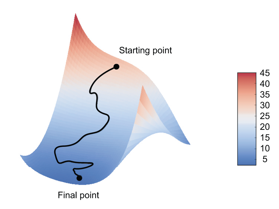
训练的时候,可能掉入局部最优解。因此SGD有很多变种。
他们更新当前W时,将之前的W也考虑其中。
如果 SGD with momentum / Adagrad / RMSprop
这些变种叫做:optimization methods或者 optimizers
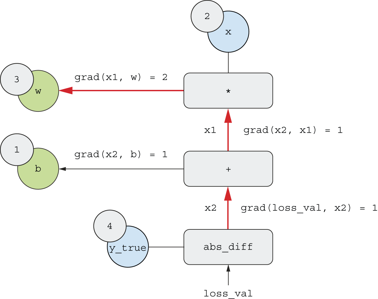
Chaining derivatives: The Backpropagation algorithm
对于多层情况,需要更新每一层的参数。
grad(loss_val, w) = grad(loss_val, x2) * grad(x2, x1) * grad(x1, w).
可以根据复合函数的导数,类似来推导:

这里就不做详细的推导了。